|
||
| Appendix
A: Chaos and Measurement
|
||
| Measurement of Initial Conditions
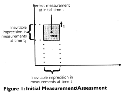
In Appendix Figure 1 we are
considering that the initial condition of an organization is measured or assessed
according to two variables X (e.g., current FTE's) and Y (e.g., number of admissions)
graphed in a coordinate system (called a phase or state space). If measurement could have
perfect accuracy, then it could be represented in the coordinate system as a "perfect
point" (see the point P(x, y) within the smaller shaded square on the left). But
because there can never be perfect accuracy in measurement, this "perfect point"
would actually have to be a two dimensional region surrounding the "perfect
point," i.e., the smaller shaded square on the left of the diagram which represents
the inevitable error or lack of knowledge or information we have about the system at t1.
The inevitable imprecision inherent in assessment means that there will always exist a
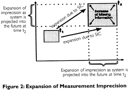
certain amount of information that is just not available at any particular time. Expansion of Measurement Imprecision
In Appendix Figure 2, we find the smaller shaded
square expanding due to sensitive dependence on initial conditions. In a strongly
nonlinear system such as chaos, the lack of perfect accuracy in initial measurements
becomes increasingly worse, in other words, the information we are missing about the
system exponentially increases. - you can see how much larger the shaded box on the right
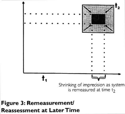
is compared to the smaller one on the left. Remeasurement at Later Time:
Consider, for instance, that instead of trying to predict
the future based on an assessment or measurement of initial conditions at some point of
time, we merely remeasure or reassess a system at a later time (t2) in the same way that
we measured or assessed the system at the initial time. We again see the larger shaded
square on the right, which originally represented the growth in inaccuracy (or lack of
information or knowledge), but, now the remeasurement at time (t2) shrinks the region of
imprecision that had been expanded when we, at an earlier time, had projected the initial
assessment into the future. The remeasurement shrinks the expanded region because it is an
actual measurement, not a projection from a past state which had to expand the region due
to sensitive dependence on initial conditions in this strongly nonlinear system.
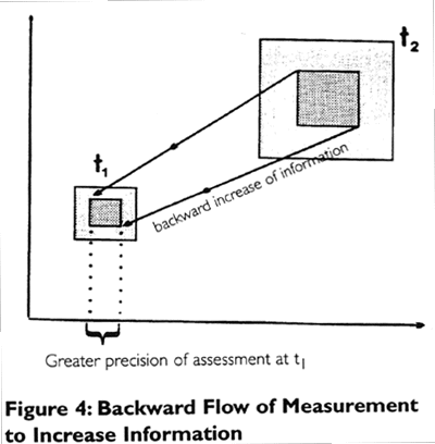
Remeasurement by itself, however, is not sufficient to generate greater information or
knowledge of the system; we also need to relate the new to the old measurement; see
Appendix Figure 4: Backward Flow of Decrease of Ignorance:
Since the remeasurement of the system at the later time shrinks the right hand expanded square to a smaller dimension, there is now greater precision or more information available. That is, our ignorance based on the earlier projection has decreased.
|
||
|
Next | Previous
Copyright © 2001, Plexus Institute Permission |